
Maxwell Equations Explained: Electricity, Magnetism and Light
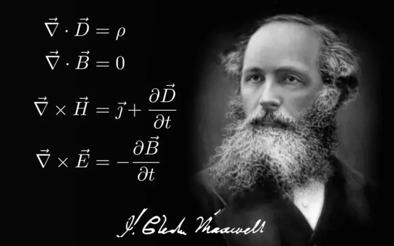
Maxwell Equations Explained: Electricity, Magnetism and Light
- The Hidden Symmetry: Electric and Magnetic Fields Can Drive Each Other
- How an Electromagnetic Wave Emerges From the Equations
- Maxwell’s Great Prediction: Light Is an Electromagnetic Wave
- Hertz Turns Maxwell’s Prediction Into an Experiment
- Why Are Maxwell Equations Written as Four Equations Today?
- Maxwell Equations in Vacuum vs. Materials
- What Maxwell Equations Actually Tell Us About Antennas
- One More Important Point: Maxwell Equations Are Not the Whole of Electromagnetism
- The Four Equations in One Picture
- Conclusion
Introduction
There are many equations that changed the course of physics, but few have united so many seemingly different phenomena into one theory as Maxwell equations.
Electricity, magnetism and light once appeared to belong to different parts of physics. Scientists could describe electric charges, magnetic effects and optical phenomena separately, but they lacked a single framework that explained how these effects were connected.
James Clerk Maxwell changed that picture.
Building on experimental and theoretical work by scientists such as Charles-Augustin de Coulomb, Hans Christian Ørsted, André-Marie Ampère and Michael Faraday, Maxwell developed a mathematical theory of electromagnetism. One of its most remarkable consequences was that electromagnetic fields can propagate through empty space as waves—and that the predicted wave speed is the speed of light.
Today, Maxwell equations remain a foundation of classical electromagnetism. They are used to understand everything from electromagnetic induction and wave propagation to antennas, RF systems, radar and wireless communication.
But what do the equations actually say?
To understand their importance, it helps to follow the problem that physicists were trying to solve.
1. How Electricity and Magnetism Became Connected
For a long time, electricity and magnetism seemed to be separate natural phenomena.
Scientists had observed electric effects and magnetic effects for centuries, but there was no clear reason to believe that one was related to the other.
That changed in the 19th century.
Ørsted: Electric Current Can Produce a Magnetic Effect
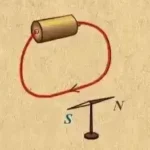
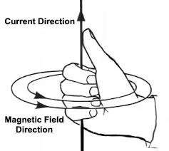
In 1820, Danish physicist Hans Christian Ørsted observed that a compass needle moved when an electric current flowed through a nearby wire.
The experiment was simple, but the implication was profound: an electric current can produce a magnetic effect.
Electricity and magnetism were not independent after all.
Ørsted’s observation quickly attracted attention across Europe. André-Marie Ampère investigated the forces associated with electric currents and developed mathematical descriptions of their magnetic effects. The emerging field of electromagnetism was beginning to take shape.
But one major question remained.
If electric current could produce a magnetic effect, could a magnetic effect produce electricity?
Faraday: Changing Magnetic Fields Can Produce an Electromotive Force
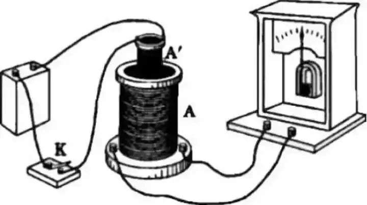
Michael Faraday answered that question through experiments carried out in 1831.
Faraday showed that changing magnetic conditions could induce an electromotive force in a nearby circuit. In a closed conducting circuit, this can drive an induced current. His experiments established the phenomenon now known as electromagnetic induction and provided the physical basis for electrical generators and transformers.
Faraday’s contribution went beyond the discovery of induction.
He developed the idea that electric and magnetic effects should be understood in terms of fields distributed through space. Instead of thinking only about forces acting between separated objects, physicists could begin thinking about what was happening in the space around charges, currents and magnets.
This field-based picture became extremely important.
Faraday had the physical intuition and experimental evidence. Maxwell would provide the mathematical framework.
2. Maxwell's Central Idea: Electromagnetism Is One System
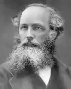
James Clerk Maxwell studied Faraday’s work and recognized that the concept of a field could be expressed mathematically.
His contribution was not simply to collect four existing equations.
Maxwell brought together several existing laws, reformulated electromagnetic theory mathematically, and added a crucial term to Ampère’s law. That additional term became known as the displacement current.
This correction was essential because it made the theory consistent for time-varying electric fields and completed the symmetry between changing electric and magnetic fields.
Maxwell presented his electromagnetic theory in the 1860s, including his 1864 paper A Dynamical Theory of the Electromagnetic Field, and developed it further in his 1873 A Treatise on Electricity and Magnetism.
The result is what we now call Maxwell equations.
3. What Are Maxwell Equations?
In modern vector calculus, Maxwell equations are commonly written as four differential equations.
For classical electromagnetism in vacuum, a standard form is:
1. Gauss's Law for Electricity
∇ · E = ρ/ε₀
2. Gauss's Law for Magnetism
∇ · B = 0
3. Faraday's Law
∇ × 𝐄 = -∂𝐁/∂t
4. Ampère-Maxwell Law
∇ × 𝐁 = μ₀𝐉 + μ₀ε₀ ∂𝐄/∂t
These four equations contain a huge amount of physical information.
Before looking at them individually, it is worth understanding the symbols.
What Do E, B, ρ and J Mean?
E is the electric field. It describes the electric force that a charged particle would experience per unit charge at a given location.
B is the magnetic flux density, measured in teslas. In introductory discussions, people often call B simply the magnetic field. In more precise electromagnetic engineering language, however, B and H are different quantities.
ρ is the electric charge density.
J is the electric current density.
ε₀ is the permittivity of free space, while μ₀ is the permeability of free space.
The symbols may look abstract at first, but the physical relationships behind them are surprisingly simple.
4. The First Equation: Electric Charges Create Electric Fields
Gauss's Law for Electricity
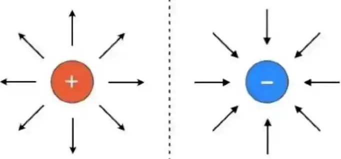
The key idea is: Electric charge is a source of electric field.
A positive charge produces an electric field that points outward. A negative charge produces an electric field that points inward.
Gauss’s law tells us something deeper than that visual picture. It connects the amount of electric charge enclosed by a closed surface with the net electric flux passing through that surface.
- Differential form: ∇ · E = ρ/ε₀
- Integral form: ∮ E · dA = Q_enc/ε₀
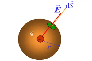
Imagine surrounding a charge with an invisible closed surface.
If the surface encloses more net electric charge, more electric flux passes outward through it. If the enclosed net charge is zero, the total electric flux through the closed surface is zero, even though electric fields may still exist locally on the surface.
This is an important point: Gauss’s law describes the divergence of the electric field. It does not mean that every electric field must point directly away from a charge.
For highly symmetric situations, however, Gauss’s law becomes a powerful way to calculate electric fields. It is closely related to Coulomb’s law, but Gauss’s law gives a broader field-based description.
5. The Second Equation: Magnetic Fields Have No Known Isolated Sources
Gauss's Law for Magnetism
∇ · B = 0
At first glance, this looks almost too simple. But it expresses an important structural property of classical magnetism:
Magnetic field lines do not begin or end at isolated magnetic charges.
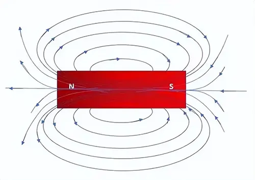
For an ordinary bar magnet, magnetic field lines form continuous loops. If you cut the magnet in half, you do not obtain a standalone north pole and a standalone south pole. You obtain two smaller magnets, each with both poles.
The integral form makes the idea especially clear:
∮_S B · dA = 0
The net magnetic flux through any closed surface is zero.
This does not prove that magnetic monopoles can never exist in any extension of physics. It means that no magnetic monopoles have been observed in classical electromagnetism, and the standard Maxwell equations describe the magnetic field without a magnetic-charge source term.
That distinction is important when discussing the equation scientifically.
6. The Third Equation: Changing Magnetic Fields Create Circulating Electric Fields
Faraday's Law of Electromagnetic Induction
∇ × E = -∂B/∂t
This is Faraday’s law in differential form.
The key idea is:
A changing magnetic field produces a circulating electric field.
This is different from saying that a magnetic field automatically creates an electric current. A changing magnetic field creates an electric field. Whether that electric field produces a measurable current depends on the conducting path and the electrical properties of the system.
The integral form is:
∮ E · dl = -dΦ_B/dt
where Φ_B is the magnetic flux through the surface bounded by the loop.
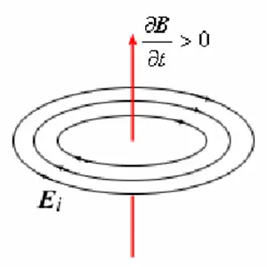
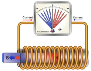
The minus sign represents Lenz’s law: the induced electromagnetic effect acts in a direction that opposes the change responsible for the induction.
This equation explains the operating principle of generators and transformers.
When a generator changes the magnetic flux linked with a conducting circuit, an electromotive force appears. When the magnetic flux through a transformer winding changes, an electromotive force is induced in the winding.
The important word is change. A perfectly static magnetic field does not, by itself, produce the circulating electric field described by Faraday’s law.
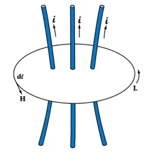
7. The Fourth Equation: Electric Current and Changing Electric Fields Create Magnetic Fields
Ampère-Maxwell Law
∇ × B = μ₀J + μ₀ε₀ ∂E/∂t
This equation contains two sources of magnetic-field circulation.
The first is ordinary electric current: μ₀J
The second is the term Maxwell added: μ₀ε₀ ∂E/∂t
This second contribution is associated with the displacement current.
And this is where Maxwell’s theoretical contribution becomes particularly important.
8. Why Maxwell Needed the Displacement Current
Consider a capacitor connected to a circuit and being charged.
Current flows through the wire toward the capacitor plate. But no ordinary charge carriers cross the insulating gap between the plates.
Now imagine applying Ampère’s original law around a closed loop surrounding the wire.
One possible surface bounded by the loop cuts through the wire and encloses a conduction current.
Another possible surface stretches between the capacitor plates and does not contain the conduction current.
The same loop would therefore appear to enclose two different currents.
That is a problem.
A physical law cannot depend on which imaginary surface we choose.
Maxwell solved this inconsistency by recognizing that the changing electric field between the capacitor plates contributes to the magnetic-field relationship.
He introduced the displacement-current term:
I_d = ε₀ dΦ_E/dt
The corrected law becomes:
∮ B · dl = μ₀I + μ₀ε₀ dΦ_E/dt
The displacement current is not simply “electrons flowing through empty space.”
That is one of the most common oversimplifications.
It is a term in electromagnetic theory that accounts for the effect of a time-varying electric field in the same magnetic-field relation as ordinary current.
That small mathematical correction has enormous consequences.
It completes the coupling between electric and magnetic fields.
9. The Hidden Symmetry: Electric and Magnetic Fields Can Drive Each Other
Now look at the two equations that contain time derivatives:
∇ × E = -∂B/∂t
and
∇ × B = μ₀J + μ₀ε₀ ∂E/∂t
Ignore charges and ordinary currents for a moment and consider empty space.
The equations reduce to:
∇ × E = -∂B/∂t
∇ × B = μ₀ε₀ ∂E/∂t
Now the structure becomes clear.
A changing magnetic field is connected to an electric field.
A changing electric field is connected to a magnetic field.
This mutual coupling is the key to understanding electromagnetic waves.
10. How an Electromagnetic Wave Emerges From the Equations
Suppose a changing electric field appears in space.
That changing electric field contributes to a magnetic field.
The changing magnetic field then generates another electric-field variation.
That electric-field variation produces another magnetic-field variation farther away.
The disturbance can therefore propagate through space.
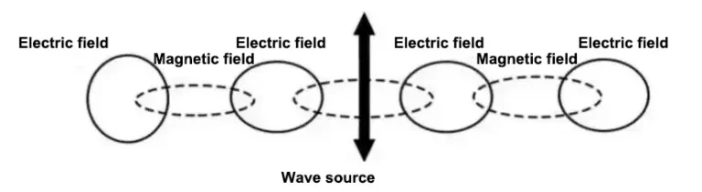
Maxwell’s equations lead directly to a wave equation for the electric and magnetic fields.
For the electric field in source-free vacuum:
∇²E = μ₀ε₀ ∂²E/∂t²
An equivalent equation holds for the magnetic field:
∇²B = μ₀ε₀ ∂²B/∂t²
Now compare this with the standard form of a wave equation:
∇²Ψ = (1/v²) ∂²Ψ/∂t²
From this comparison, the wave velocity follows as:
v = 1/√(μ₀ε₀)
This velocity is the speed of electromagnetic waves in vacuum.
Its numerical value is approximately:
3.00 × 10⁸ m/s
which is the speed of light in vacuum.
This was a remarkable theoretical result.
Maxwell did not start with a statement that “light must be an electromagnetic wave.”
The mathematical structure of electromagnetic theory led him there.
11. Maxwell's Great Prediction: Light Is an Electromagnetic Wave
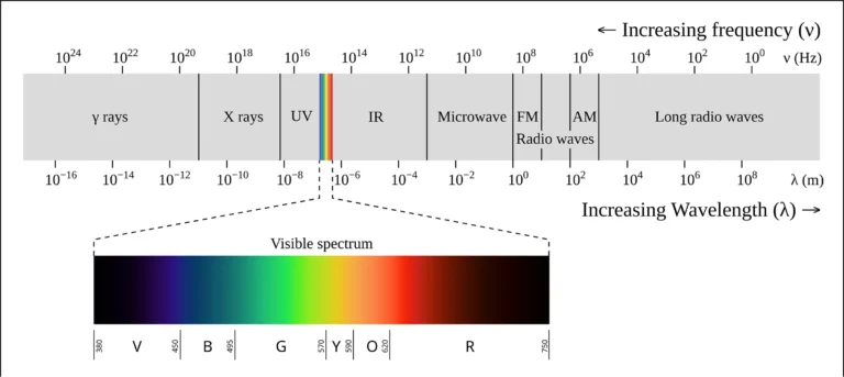
Once Maxwell found that electromagnetic disturbances should propagate at the same speed as light, the connection became difficult to ignore.
His conclusion was that light is an electromagnetic phenomenon.
Visible light is therefore not fundamentally separate from radio waves, microwaves, infrared radiation, ultraviolet radiation, X-rays or gamma rays.
They all belong to the electromagnetic spectrum.
Their frequencies, wavelengths and photon energies differ, but their classical electromagnetic fields obey the same fundamental equations.
This was one of the deepest unifications in classical physics.
12. Hertz Turns Maxwell's Prediction Into an Experiment
A mathematical prediction still needs experimental testing.
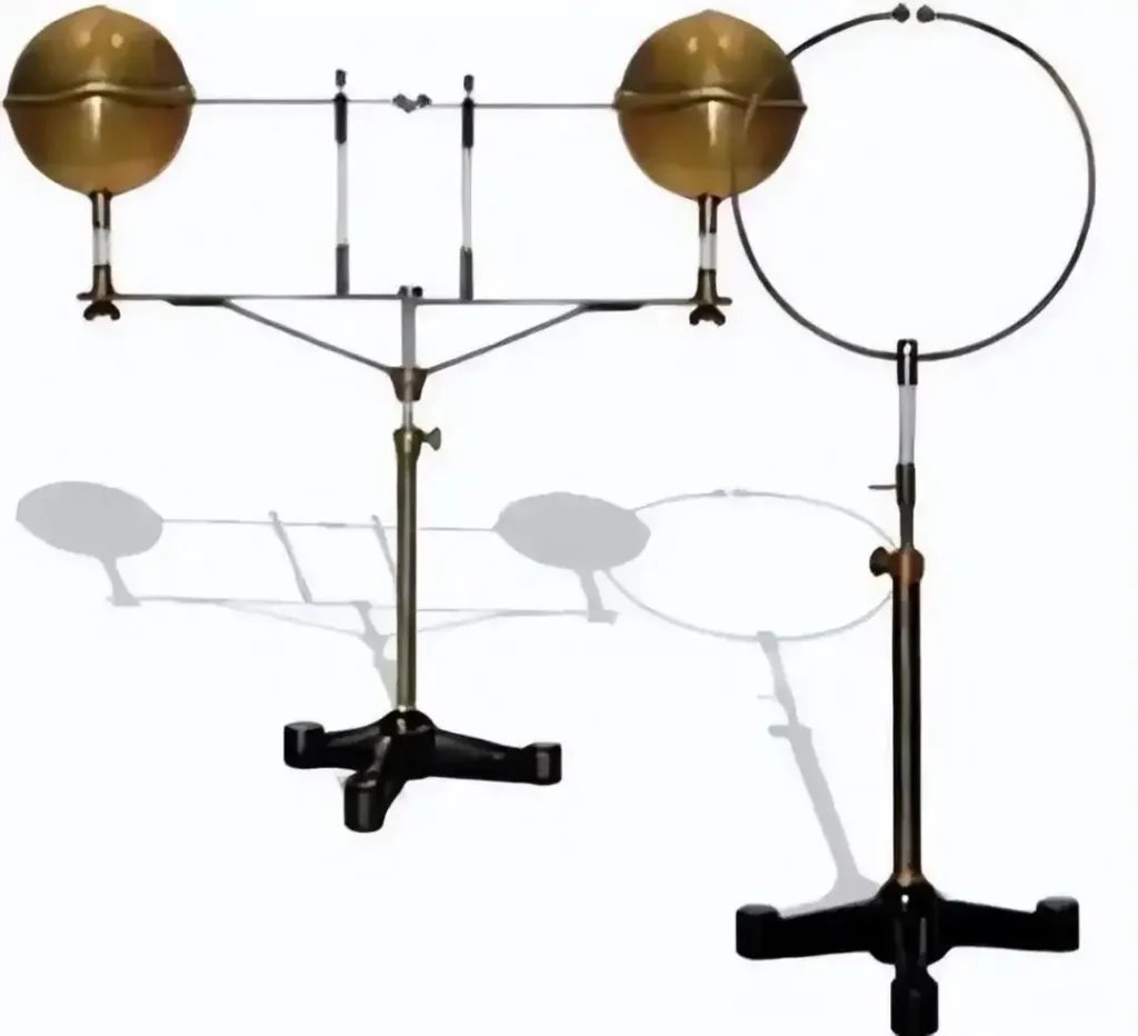
That test came from German physicist Heinrich Hertz.
During experiments in the late 1880s, Hertz generated and detected electromagnetic waves in the laboratory and demonstrated properties such as reflection and interference that were consistent with Maxwell’s theory. His work provided experimental confirmation that electromagnetic waves really existed.
The historical sequence matters:
Maxwell developed the theory → the theory predicted electromagnetic waves → Hertz detected and studied those waves experimentally.
Maxwell himself died in 1879, before Hertz’s experimental work.
This is one reason the Maxwell-Hertz story is so important in physics. It illustrates a powerful relationship between mathematical theory and experiment.
A theory can reveal something that no one has directly observed yet.
An experiment can then test whether nature actually behaves as the theory predicts.
13. Why Are Maxwell Equations Written as Four Equations Today?
There is an interesting historical detail behind the name “Maxwell equations.”
Maxwell did not originally write the theory as the four compact vector equations found in modern textbooks.
His original formulation used a much larger mathematical system, with equations expressed largely through component notation and other mathematical structures.
Later, Oliver Heaviside and J. Willard Gibbs developed vector-calculus formulations that made electromagnetic theory far more compact and practical. The familiar modern four-equation form emerged from this later mathematical development.
So when we say “Maxwell equations,” we mean the modern formulation of the electromagnetic theory that Maxwell developed, rather than four equations that Maxwell himself wrote down in exactly their present textbook appearance.
The underlying physical content is Maxwell’s.
The compact notation came later.
This distinction is more historically accurate and also explains why the equations look much cleaner today than Maxwell’s original mathematical presentation.
14. Maxwell Equations in Vacuum vs. Materials
The four equations are often presented in vacuum form using E and B.
In electromagnetic engineering, especially when dealing with dielectrics, conductors and other materials, engineers commonly work with:
E: electric field
D: electric displacement field
B: magnetic flux density
H: magnetic field intensity
For example, a common macroscopic form is:
∇ · D = ρ_f
∇ · B = 0
∇ × E = -∂B/∂t
∇ × H = J_f + ∂D/∂t
where ρ_f and J_f represent free charge and free current densities.
The relationships between these quantities and the material properties depend on the medium.
For a simple linear isotropic material, for example:
D = εE
B = μH
This distinction becomes important in practical antenna and RF problems because real antennas are surrounded by materials, substrates, radomes, enclosures and sometimes nearby conductors.
The electromagnetic field does not behave only according to the antenna geometry. It also depends on the electromagnetic properties of the surrounding environment.
15. What Maxwell Equations Actually Tell Us About Antennas
For antenna engineers, Maxwell equations are much more than a piece of physics history.
An antenna is an electromagnetic device.
When an alternating current and voltage excite an antenna structure, the resulting time-varying electric and magnetic fields interact and propagate according to Maxwell’s equations.
That connection gives rise to many of the quantities engineers use every day.
Electromagnetic waves in free space satisfy:
c = f λ
where c is the speed of light, f is frequency and λ is wavelength.
As frequency increases, wavelength decreases.
That is one reason antenna dimensions are strongly connected to operating frequency.
A 915 MHz antenna and a 5.8 GHz antenna may both be RF antennas, but they operate on very different electromagnetic length scales.
The electric field of an electromagnetic wave has a direction.
That direction can remain approximately fixed, rotate, or follow a more general time-varying path.
This gives rise to linear, circular and elliptical polarization.
For example, in a circularly polarized wave, the electric-field vector rotates as the wave propagates.
This is why antenna polarization is not simply a mechanical property of the antenna. It describes the behavior of its radiated electromagnetic field.
An antenna does not necessarily radiate the same amount of energy in every direction.
Its geometry determines how electromagnetic energy is distributed in space.
The resulting directional behavior is described by quantities such as radiation pattern, beamwidth, front-to-back ratio and gain.
These are practical engineering descriptions of solutions to electromagnetic field problems.
Maxwell equations describe fields, but engineers also need circuit-level quantities to analyze how efficiently RF energy moves between components.
This is where impedance becomes important.
A mismatch between a source, transmission line and antenna causes part of the incident electromagnetic energy to be reflected.
That leads to familiar RF parameters such as reflection coefficient, return loss and VSWR.
These concepts are not separate from electromagnetism. They are practical engineering descriptions of what happens when electromagnetic waves encounter an impedance discontinuity.
16. One More Important Point: Maxwell Equations Are Not the Whole of Electromagnetism
It is tempting to think that the four equations explain everything about electromagnetic forces.
Strictly speaking, Maxwell equations describe how electromagnetic fields are generated and how they evolve.
To determine the force acting on a charged particle, we also use the Lorentz force law:
F = q(E + v × B)
So Maxwell equations and the Lorentz force law play complementary roles.
Maxwell equations describe the electromagnetic field.
The Lorentz force describes how a charged particle responds to that field.
This distinction becomes important when studying the motion of charges, currents and matter in electromagnetic fields.
17. The Four Equations in One Picture
After all the mathematics, the physical picture can be reduced to four ideas:
Gauss’s Law for Electricity
Electric charge determines the divergence of the electric field.
Gauss’s Law for Magnetism
Magnetic flux has no net divergence in classical electromagnetism; no magnetic monopoles have been observed.
Faraday’s Law
A changing magnetic field produces a circulating electric field.
Ampère-Maxwell Law
Electric current and a changing electric field contribute to a circulating magnetic field.
Put the last two together and the deeper structure appears:
Changing electric field → magnetic field
Changing magnetic field → electric field
Under the right conditions, that mutual coupling produces an electromagnetic wave that can travel through vacuum.
That is the central idea behind Maxwell equations.
Conclusion
Before the development of electromagnetic field theory, electricity, magnetism and light belonged to seemingly separate areas of natural philosophy.
The experiments of Ørsted and Faraday showed that electricity and magnetism were connected. Ampère and other researchers developed quantitative descriptions of their interactions. Maxwell then built a broader mathematical theory and introduced the displacement-current term that completed the dynamic relationship between electric and magnetic fields.
The theory led to a remarkable prediction: electromagnetic fields can propagate as waves through empty space, with a speed determined by the electromagnetic properties of vacuum:
c = 1/√(μ₀ε₀)
That speed is the speed of light.
Hertz later confirmed the existence of electromagnetic waves experimentally.
The lasting significance of Maxwell equations is therefore not simply that they are mathematically elegant.
They show that phenomena that appear different at first can belong to the same physical system.
Electricity, magnetism and light are not three unrelated stories.
They are different aspects of electromagnetism.
And whenever an antenna radiates, a wireless signal propagates, or an RF system exchanges electromagnetic energy, the physics described by Maxwell equations is still at work.
You may also like
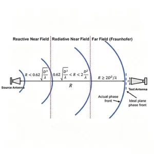
Learn how antenna near field and far field regions work, how to calculate far-field distance, and why antenna size matters.
This article introduces the Antenna Basics, Concepts & Theory, the fundamentals of antenna theory and related knowledge.

Antenna Array Fundamentals Explained, covering dipoles, antenna elements, array gain, beamforming, and 5G basics.
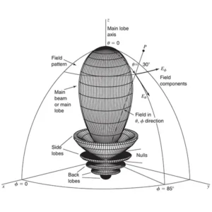
This article is about the Antenna Radiation Patterns Explained, it contain a Visual Guide to 85 Antenna Types.
Contact
We are always ready to serve you.
Please feel free to contact us
for any antenna inquiry or requirement.
Leave us a message in the form below and
we will get back to you within 24 hours.