Why Is 50 Ohms the Standard Impedance in RF Systems?

Introductions

In RF and microwave engineering, 50 ohms appears almost everywhere. You will find it in coaxial cables, SMA and N-Type connectors, VNA ports, RF amplifiers, filters, attenuators, switches, PCB transmission lines, and antenna interfaces.

But why 50 ohms? Is there something special about this number, or is it simply a convention engineers have followed for decades?

The answer is more interesting than it first appears. 50 ohm RF impedance is not a physical constant or a universally optimal value. It emerged from a practical engineering trade-off involving power handling, transmission loss, physical dimensions, manufacturing, and system compatibility.

Understanding why 50 ohms became the dominant RF standard also makes it easier to understand impedance matching, coaxial cables, antennas, VSWR, and RF system design.

I. What Is Characteristic Impedance?

At low frequencies, it is often enough to think of a circuit in terms of voltage, current, resistance, and capacitance.

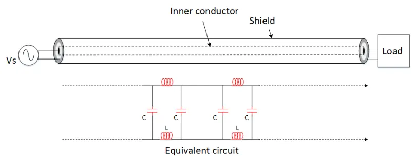
At RF frequencies, however, electrical signals behave as electromagnetic waves traveling along transmission lines. The geometry and materials of the transmission line determine how voltage and current relate as the wave propagates.

This relationship is called characteristic impedance, usually written as Z₀.

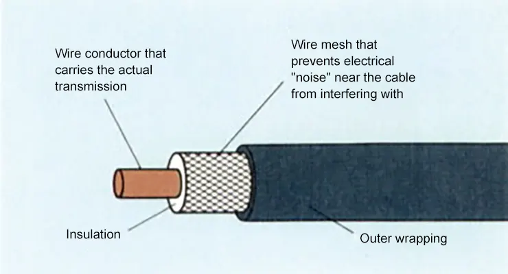
For an ideal coaxial cable, the characteristic impedance can be approximated by: Z₀ = (60 / √εᵣ) × ln(b/a)

where Z₀ is the characteristic impedance, εᵣ is the relative permittivity of the dielectric, a is the radius of the inner conductor, b is the inner radius of the outer conductor.

For an air-filled coaxial cable, where εᵣ is approximately 1: Z₀ ≈ 60 × ln(b/a)

This equation shows an important point: impedance is determined by the physical structure of the transmission line, not simply by the material of the conductor. Changing the conductor dimensions or dielectric material changes the characteristic impedance.

So why did engineers eventually settle on 50 ohms?

II. Why Do Different Impedances Have Different Advantages?

A coaxial cable has to satisfy several competing requirements.

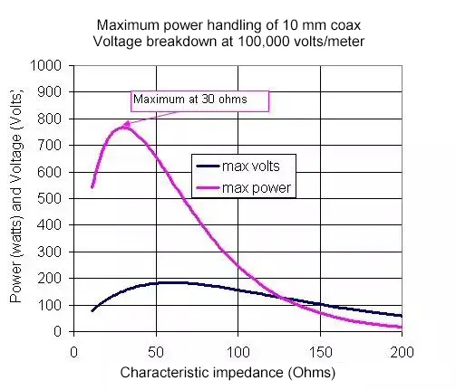
For an air-dielectric coaxial cable, classical electromagnetic analysis identifies several useful impedance regions. Around 30 ohms, the geometry provides high power-handling capability.
Around 60 ohms, the cable can support relatively high voltage.
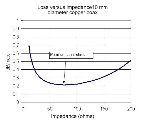
Around 77 ohms, conductor loss reaches a classical minimum under idealized air-coax conditions.

These values are not arbitrary. They result from how the electromagnetic field is distributed inside the coaxial structure and how that field interacts with the conductors.

This creates an engineering trade-off: If you optimize the cable for one characteristic, you generally give something up somewhere else. And that brings us to the question: if roughly 30 ohms is favorable for power handling and roughly 77 ohms is favorable for low conductor loss, why did 50 ohms become the standard?

III. Between 30 Ohms and 77 Ohms, Why Did 50 Ohms Win?

Consider an air-dielectric coaxial cable:

A larger inner conductor reduces the b/a ratio and therefore lowers the characteristic impedance. This can improve power-handling capability under the relevant conditions, but it also introduces structural and loss trade-offs.

A smaller inner conductor increases the impedance and moves the design toward the lower conductor-loss region of an air coaxial cable. However, power handling, mechanical strength, and physical dimensions then become important concerns.

In real engineering, engineers have to balance power handling, transmission loss, physical size, manufacturing difficulty, and system compatibility.

There is a fairly wide range between 30 ohms and 77 ohms. 50 ohms sits within this range as a practical compromise. It does not favor the power-handling extreme or the low-loss extreme, but provides a balance that is easier to accept across a complete RF system.

There was also a practical manufacturing consideration.

Early coaxial structures could be built using readily available standard copper tubing. For example, a coaxial geometry using a 3/4-inch inner conductor and a 2-inch outer conductor gives a characteristic impedance of roughly 51.5 ohms under an ideal air-filled approximation. That is remarkably close to 50 ohms.

This made a value near 50 ohms practical to manufacture using available materials and dimensions, helping reduce engineering and manufacturing difficulties.

So 50 ohms was not adopted simply because it was the exact average of 30 and 77 ohms, nor because it was mathematically “perfect.” It was a practical value that satisfied electromagnetic performance, available materials, manufacturing considerations, and system requirements.

Over time, that practical compromise became a widely accepted RF interface standard.

IV. The Real Importance of 50 Ohms: System Compatibility

The biggest advantage of 50 ohms today is that all RF components have optimal compatibility at 50 ohms.

Consider a typical RF signal path: Transmitter → Amplifier → Filter → Switch → Cable → Connector → Antenna

If these interfaces are designed around a common 50-ohm system impedance, engineers can connect components from different manufacturers with predictable RF behavior.

A 50-ohm signal generator can drive a 50-ohm cable. That cable can connect to a 50-ohm filter, attenuator, switch, or antenna.

The same standard also allows RF test equipment such as vector network analyzers and power meters to operate within a common impedance environment. This is why 50 ohms has become more than a cable specification. It is effectively a common engineering language for RF interfaces.

V. What Happens When the Impedance Does Not Match?

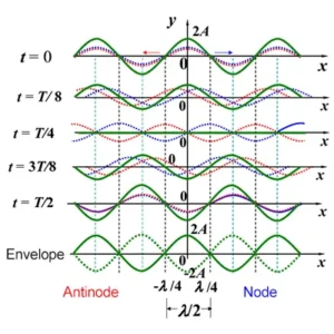
When a transmission line encounters a load with a different impedance, part of the RF wave is reflected back toward the source.

The reflection coefficient is: Γ = (ZL − Z₀) / (ZL + Z₀)

If the load impedance equals the characteristic impedance: ZL = Z₀, then: Γ = 0, there is no load mismatch reflection.

This is the basic principle behind RF impedance matching.

Engineers commonly describe the amount of reflection using parameters such as VSWR, Return Loss, and S11.

For example, an antenna may specify: Impedance: 50 Ω, VSWR: ≤ 1.5

This does not mean the antenna has a perfect 50-ohm impedance at every frequency. Instead, it means the antenna is designed to present an impedance close enough to the 50-ohm system over its specified operating range.

Poor matching can reduce the power delivered to an antenna and increase reflected power toward the RF front end. In higher-power systems, excessive reflected power can also place additional stress on RF components.

VI. Why Do Antennas Commonly Use 50 Ohms?

It is important to understand that antennas are not naturally 50 ohms. An antenna’s input impedance depends on its geometry, operating frequency, feeding method, surrounding environment, and installation conditions.

For example, an ideal center-fed half-wave dipole in free space has an input resistance of roughly 73 ohms, not 50 ohms.

So why do commercial RF antennas commonly specify 50-ohm impedance?

Because they are designed to work with the rest of the RF system. RF modules, coaxial cables, connectors, test equipment, and many radio interfaces use 50 ohms. Designing the antenna interface around the same impedance simplifies integration and reduces the need for additional matching.

Therefore, 50 ohms is a common RF system interface standard, not an inherent property of antennas.

VII. Why Is 75 Ohms Also Common?

If 50 ohms were always the best choice, 75-ohm systems would not exist. But different applications have different priorities.

In many video, broadcast, and CATV distribution systems, low transmission loss is more important than high power handling. A higher characteristic impedance can be advantageous for reducing conductor loss under classical coaxial assumptions. That is one reason 75-ohm coaxial cable became widely used in video and cable distribution applications.

This is also why comparing 50 ohm vs 75 ohm is not really about deciding which impedance is “better.” They were developed around different system requirements.

50 ohms became dominant in many RF and wireless systems where power handling, loss, component compatibility, and general-purpose RF use all mattered.
75 ohms became particularly common in applications where low loss and signal distribution were more important.

VIII.What About 93 Ohms, 100 Ohms, and 120 Ohms?

50 and 75 ohms are not the only impedance values used in electrical systems.

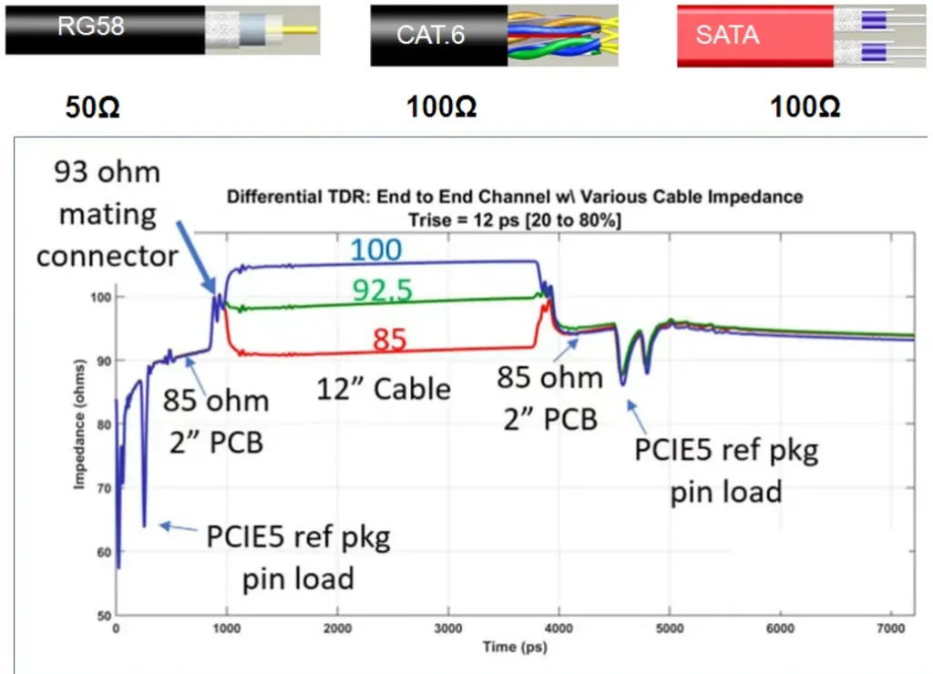
For example, 93-ohm RG-62 coaxial cable was historically used in applications where low capacitance per unit length was useful.

High-speed digital interfaces commonly use 100-ohm differential impedance.

It is important not to think of 100-ohm differential impedance as simply “two 50-ohm traces added together.” Differential impedance depends on the geometry and electromagnetic coupling between the two conductors, including trace width, spacing, dielectric thickness, and dielectric constant.

Other interfaces, such as RS-485, commonly use 120-ohm differential transmission lines.

These examples demonstrate an important principle:

The right impedance depends on the transmission-line structure and the requirements of the system.

IX. Does Every RF Circuit Have to Be 50 Ohms?

No. 50 ohms is primarily a system and interface standard.

Inside an RF amplifier, for example, the optimum impedance presented to an active device may be significantly different from 50 ohms. The designer can use a matching network to transform the device’s optimum impedance to the 50-ohm impedance required by the external RF system.

This distinction is important. A component can have an internal operating impedance that is very different from 50 ohms while still providing a 50-ohm input or output interface. So when you see “50 ohms” on an RF datasheet, it does not necessarily describe every electrical point inside the device.

X. Why Has 50 Ohms Survived for So Long?

Once an impedance becomes a widely adopted standard, changing it becomes extremely difficult.

Cable manufacturers produce 50-ohm coaxial cables.

Connector manufacturers produce 50-ohm connectors.

RF component manufacturers design amplifiers, filters, switches, attenuators, and other components around 50-ohm interfaces.

Test-equipment manufacturers build VNAs, signal generators, spectrum analyzers, and power meters around the same standard.

The entire ecosystem becomes interconnected.

As a result, 50 ohms provides something extremely valuable: predictable interoperability. Engineers do not have to redesign the impedance interface every time they connect two RF components.

That standardization is one of the main reasons 50 ohms has remained dominant for so many decades.

So, Why 50 Ohms?

There is no single equation that says RF systems must use 50 ohms. The value emerged from a combination of electromagnetic theory, engineering trade-offs, available materials, manufacturing practicality, and historical standardization.

For classical air-dielectric coaxial structures, around 30 ohms is associated with high power-handling capability, while around 77 ohms corresponds to a low conductor-loss region. 50 ohms sits between these extremes and provides a practical balance.

More importantly, once 50 ohms became widely adopted, an entire RF ecosystem developed around it. That is why 50 ohms remains the dominant interface impedance across much of RF and microwave engineering.

It is not a universal physical law. It is a practical engineering standard that became a common language for RF systems.

Contact

We are always ready to serve you.

Please feel free to contact us
for any antenna inquiry or requirement.

Leave us a message in the form below and
we will get back to you within 24 hours.

About Us

Airplux Technologies Limited is one professional Antenna Solution Provider which is integrating R&D, production and sales of antennas. Airplux manufactures superior quality DAS/Small Cell antennas, WiFi antennas, IOT/RFID/M2M/GPS antennas, Base Station antennas and customized antennas from 100MHz to 80GHz. We specializes in the production of custom antennas and related accessories.

Products

Working Hours

We are always ready to serve you.

Please send email to info@airpluxtec.com,
we will get back to you within 24 hours.