
Smith Chart Explained: Reading & Impedance Matching
Smith Chart Explained: Reading & Impedance Matching
Introduction
In radio frequency (RF) engineering, impedance matching plays an important role in controlling signal reflections and transferring power between connected components. Whether engineers are designing an antenna, optimizing an RF amplifier, or analyzing a transmission line, they need to understand how impedance changes with frequency and how those changes affect system performance.
The Smith Chart provides a practical way to visualize these relationships. By connecting complex impedance with reflection coefficient, the chart allows engineers to analyze transmission lines, evaluate impedance matching, and develop matching networks without repeatedly solving complicated equations.
Although modern simulation software and vector network analyzers (VNAs) can calculate impedance automatically, the Smith Chart remains a valuable tool for understanding RF behavior and making informed design decisions.
This guide explains the principles behind the Smith Chart, how to read its main features, and how to apply it to impedance matching and antenna measurements.
1. What Is a Smith Chart?
A Smith Chart is a graphical tool used in RF and microwave engineering to analyze complex impedance, reflection coefficients, and transmission line behavior. It represents these electrical relationships on a circular diagram, making it easier to interpret information that would otherwise require complex-number calculations.
The chart is commonly used in antenna design, RF circuit development, microwave network analysis, and impedance matching.
Why Is the Smith Chart Useful?
At high frequencies, the electrical behavior of a circuit becomes increasingly dependent on its physical dimensions and transmission line characteristics. Even small parasitic inductances and capacitances can influence impedance, while mismatches between connected components can cause signal reflections.
The Smith Chart helps engineers address these challenges by allowing them to:
- Determine impedance from a plotted point.
- Evaluate the magnitude and phase of a reflection coefficient.
- Understand voltage standing wave ratio (VSWR).
- Analyze how impedance changes along a transmission line.
- Design impedance matching networks using inductors, capacitors, and transmission line sections.
Instead of viewing impedance as an isolated numerical value, engineers can see how it relates to reflection and how circuit modifications move the operating point across the chart.
2. The History and Development of the Smith Chart
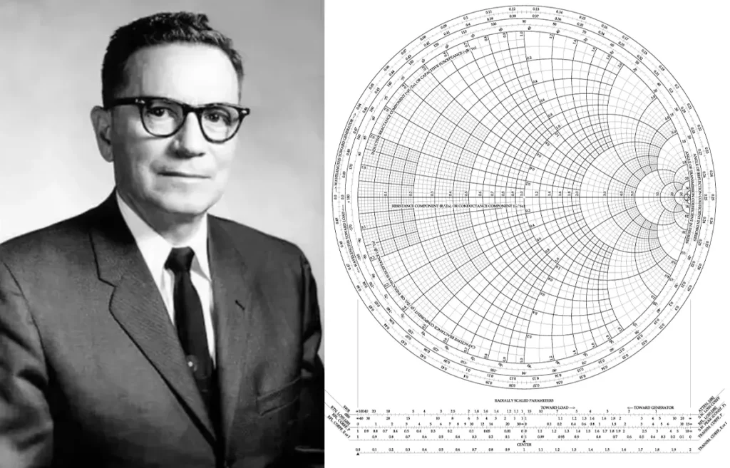
The Smith Chart was developed by American engineer Phillip H. Smith while he was working at Bell Telephone Laboratories. His work addressed the practical challenges of analyzing transmission lines and solving impedance-related problems in communication systems.
In the early days of RF engineering, engineers often relied on mathematical calculations and transmission line measurements to determine impedance and reflection characteristics. These methods could be time-consuming, particularly when repeated measurements and adjustments were necessary.
Smith developed a graphical calculation method that made these relationships easier to visualize. His work evolved from an earlier diagram into the circular format now familiar to RF engineers. In January 1939, he published his Transmission Line Calculator in Electronics magazine.
Over time, engineers widely adopted the diagram for transmission line analysis and impedance matching. Its use later expanded into electronic test equipment and computer-aided RF design.
Today, the Smith Chart appears in many VNAs and RF simulation tools. Although computers have replaced much of the manual calculation, the chart continues to help engineers understand the underlying physics of RF circuits.
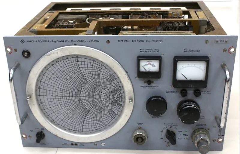
Z-graph instrument invented in 1950
3. The Basic Principles Behind the Smith Chart
To understand the Smith Chart, it helps to begin with three fundamental concepts: impedance, reflection coefficient, and normalized impedance.
3.1 Understanding Impedance in RF Systems
Impedance describes how a circuit opposes alternating current. Unlike resistance alone, impedance includes both resistive and reactive components.
Engineers express complex impedance as: Z=R+jX
Where:
- (Z) is the complex impedance, measured in ohms ((\Omega)).
- (R) is the resistance.
- (X) is the reactance.
- (j) is the imaginary unit.
Resistance represents the real component of impedance. Reactance describes the frequency-dependent effects of inductance and capacitance.
A positive reactance indicates inductive behavior, while a negative reactance indicates capacitive behavior.
The characteristic impedance of a transmission line, denoted by (Z_0), is another important parameter. Many RF systems use a nominal characteristic impedance of 50 Ω, while 75 Ω systems are also common in certain applications.
When a load impedance differs from the transmission line’s characteristic impedance, part of the incident wave reflects from the load.
3.2 What Is the Reflection Coefficient?
The voltage reflection coefficient describes the relationship between reflected and incident voltage waves at a specified reference plane.
For a load impedance (Z_L) connected to a transmission line with real characteristic impedance (Z_0), the load reflection coefficient is:
Γ_L = (Z_L − Z_0) / (Z_L + Z_0)
The reflection coefficient is a complex number. Its magnitude indicates the relative amplitude of the reflected voltage wave, while its phase describes the reflected wave’s phase relative to the incident wave under the chosen reference convention.
When the load impedance equals the characteristic impedance, the reflection coefficient is zero:
Z_L = Z_0 ⇒ Γ_L = 0
This condition represents a matched load, with no reflection at the load interface in the ideal case.
For a passive load under the usual real-reference-impedance conditions, the reflection coefficient magnitude satisfies:
|Γ_L| ≤ 1
The reflected power as a fraction of incident power is |Γ_L|², provided the incident and reflected waves are defined using the same real reference impedance.
3.3 Normalized Impedance
The Smith Chart uses normalized impedance to represent different impedance values on the same diagram.
Normalized impedance is defined as:
z = Z / Z₀ = r + jx
Where (r) and (x) are the normalized resistance and reactance, respectively.
For example, a 100 + j50 Ω load in a 50 Ω system has a normalized impedance of:
z = (100 + j50) / 50 = 2 + j1
Normalization removes the need to draw a different chart for each characteristic impedance. Engineers can use the same basic chart for 50 Ω, 75 Ω, and other systems by normalizing the relevant impedance values first.
3.4 How Impedance Maps onto the Smith Chart
The Smith Chart represents normalized impedance through its relationship with the complex reflection coefficient:
Γ = (z − 1) / (z + 1)
The reverse transformation is:
z = (1 + Γ) / (1 − Γ)
These equations establish the mathematical foundation of the chart.
The diagram uses the real and imaginary components of the reflection coefficient as its horizontal and vertical coordinates. Curves representing constant normalized resistance and constant normalized reactance are then overlaid on this plane.
Their intersections identify specific normalized impedance values.
This mapping allows engineers to move between impedance and reflection coefficient without performing the full complex-number calculation every time.
4. How to Read a Smith Chart
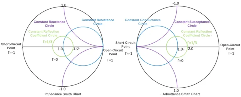
The Smith Chart may initially appear complicated because it contains many intersecting circles, arcs, and scales. However, understanding a few key features makes it much easier to use.
4.1 The Center Point: Perfect Impedance Matching
The center of the Smith Chart represents the normalized impedance:
z = 1 + j0
In a 50 Ω system, this corresponds to an impedance of 50 + j0 Ω.
At this point, the reflection coefficient is zero and VSWR equals 1. The load is matched to the reference impedance.
The center is therefore the target point in many impedance matching applications.
4.2 The Open-Circuit and Short-Circuit Points
The two endpoints of the horizontal axis represent ideal open-circuit and short-circuit conditions.
Open circuit: Located at the far right of the chart, where Γ = +1.
Short circuit: Located at the far left of the chart, where Γ = -1.
Both conditions have a reflection coefficient magnitude of 1, meaning that the entire incident wave is reflected in the ideal case. Their reflection coefficient phases differ by 180 degrees.
These points must not be confused with the center, which represents a matched load.
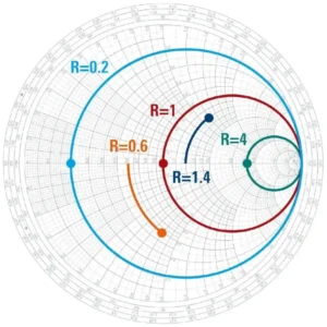
4.3 Constant Resistance Circles
Constant resistance circles represent points with the same normalized resistance (r).
Each circle corresponds to a particular resistance value. Moving along one of these circles changes the reactance while keeping the normalized resistance constant.
This feature is useful when analyzing circuits containing series components, because an ideal series reactance changes the reactance without changing the resistance.
4.4 Constant Reactance Arcs
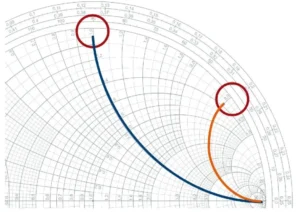
Constant reactance arcs represent points with the same normalized reactance (x).
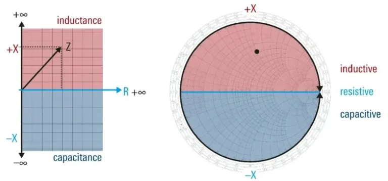
The upper half of the impedance Smith Chart represents inductive reactance, where (x>0). The lower half represents capacitive reactance, where (x<0).
The horizontal axis corresponds to zero reactance, meaning that points on this axis represent purely resistive impedances.
An impedance point is identified by the intersection of a constant resistance circle and a constant reactance arc.
4.5 A Practical Example: Reading Impedance
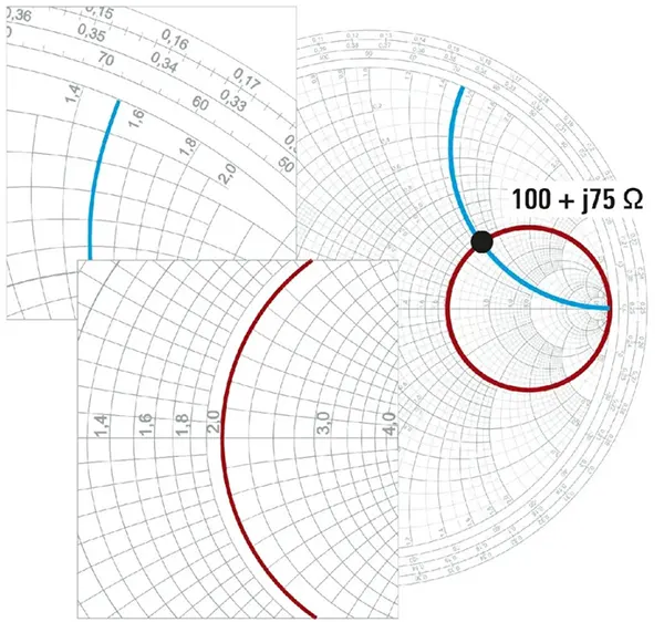
Consider a load impedance of 100 + j75 Ω in a 50 Ω system.
First, normalize the impedance:
z = (100 + j75) / 50 = 2 + j1.5
Locate the intersection of the constant resistance circle r = 2 and the constant reactance arc x = +1.5 on the Smith Chart. As shown in the figure, this point represents the load impedance.
The corresponding reflection coefficient is:
Γ = (z − 1) / (z + 1) = 0.6 + j0.2
Its magnitude is approximately 0.632, giving a VSWR of about 4.43:1.
This example shows how the Smith Chart connects normalized impedance with reflection characteristics, helping engineers evaluate impedance matching at a glance.
4.6 Understanding the VSWR Circle
A constant VSWR circle is centered on the Smith Chart’s origin.
For a given reflection coefficient magnitude, every point on this circle has the same VSWR. Along an ideal, uniform, lossless transmission line, the impedance changes with position, but the reflection coefficient magnitude remains constant.
The relationship between reflection coefficient magnitude and VSWR is:
VSWR = (1 + |Γ|) / (1 − |Γ|)
A VSWR of 1:1 indicates a perfect match. Higher values indicate a greater degree of mismatch.
The VSWR circle helps engineers visualize how the impedance presented by a transmission line changes as the observation point moves, even though the reflection magnitude remains unchanged.
4.7 Reading the Wavelength Scales
Many Smith Charts include wavelength scales around the outer edge. These scales help engineers determine how far they need to move along a transmission line to reach a particular impedance.
For a uniform, lossless transmission line, moving toward the generator rotates the reflection coefficient clockwise on the conventional Smith Chart. Moving toward the load rotates it in the opposite direction.
A movement of one-half wavelength corresponds to a complete 360-degree rotation of the reflection coefficient phase. Consequently, the impedance pattern repeats every half wavelength.
This relationship is particularly useful when designing transmission line sections and stub matching networks.
5. How to Use the Smith Chart for Impedance Matching
Impedance matching is one of the most important applications of the Smith Chart. It allows engineers to determine how circuit elements or transmission line sections can transform a load impedance toward a desired target.
5.1 The Goal of Impedance Matching
In many RF systems, engineers want a load to present an impedance equal to the transmission line’s characteristic impedance at a specified reference plane.
For a 50 Ω system, the target is typically:
Z_in = 50 + j0 Ω
On the Smith Chart, this corresponds to the center point.
A matching network can transform a load impedance to the desired input impedance at a particular frequency. However, a match at one frequency does not necessarily guarantee a good match across a wide frequency range.
It is also important to distinguish matching a load to a transmission line from conjugate matching a source and load for maximum available power transfer. The appropriate condition depends on the circuit and its design objectives.
5.2 Series Inductors and Capacitors
Adding an ideal reactive component in series changes the reactance while leaving the resistance unchanged.
A series inductor adds positive reactance:
X_L = 2πfL
A series capacitor adds negative reactance:
X_C = −1 / (2πfC)
On the impedance Smith Chart, these changes move the operating point along a constant resistance circle.
The engineer can use this relationship to identify the reactance required to move toward the target impedance, then calculate the corresponding component value at the design frequency.
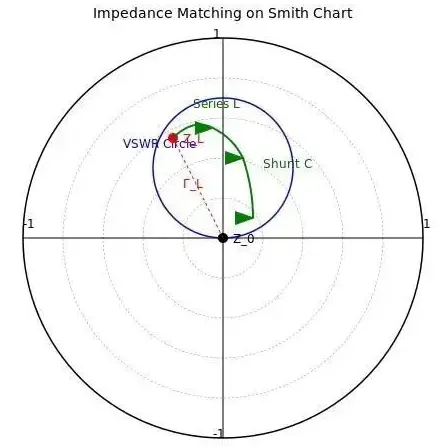
5.3 Shunt Components and the Admittance Smith Chart
Parallel components are often easier to analyze using admittance rather than impedance.
Admittance is the reciprocal of impedance:
Y = 1 / Z = G + jB
Here, (G) represents conductance and (B) represents susceptance.
When an ideal reactive component is connected in parallel, it changes susceptance while leaving conductance unchanged. Engineers can therefore use an admittance Smith Chart, or convert between impedance and admittance on a combined chart.
This distinction is important: series elements are commonly analyzed in the impedance representation, while parallel elements are often analyzed in the admittance representation.
5.4 Common Impedance Matching Networks
Several matching network configurations are widely used in RF engineering.
L-type networks use two reactive elements. Their topology depends on the load impedance and the required transformation. They are common in single-frequency and relatively narrowband applications.
Pi and T networks use three reactive elements and provide additional flexibility in impedance transformation and circuit design. They may also help engineers control network Q and other design constraints.
Quarter-wave transformers use a transmission line section with an electrical length of one-quarter wavelength at the design frequency to transform a suitable load resistance. Their performance depends on frequency and the impedances involved.
Stub matching networks use open- or short-circuited transmission line sections to introduce the required reactance or susceptance. The Smith Chart makes it easier to determine suitable line positions and electrical lengths.
No single network is optimal for every situation. Component availability, operating bandwidth, insertion loss, power handling, and physical layout all influence the final design.
5.5 A Practical Matching Workflow
A typical impedance matching process follows these steps:
Define the operating frequency or frequency band and the reference impedance.
Obtain the load impedance from measurement, simulation, or a reliable circuit model.
Normalize the impedance and locate its position on the Smith Chart.
Choose an appropriate matching topology based on the target impedance and design constraints.
Determine component values or transmission line dimensions.
Verify the design through simulation and measurement, then adjust the network if necessary.
The Smith Chart supports this process by making impedance transformations easier to visualize. Final component selection still requires appropriate calculations and practical validation.
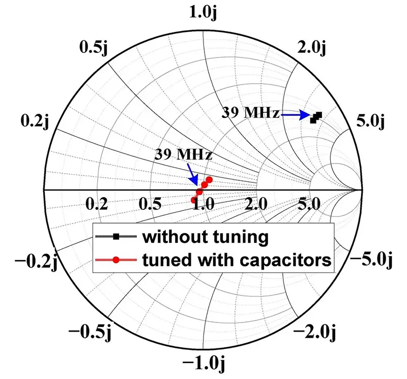
6. Using a Smith Chart for Antenna Measurements
Antenna impedance matching is an important application of the Smith Chart because an antenna’s input impedance often varies with frequency.
Engineers use the chart to examine that variation, identify potential matching requirements, and evaluate whether the antenna presents the intended impedance to its RF system.
6.1 Measuring Antenna Impedance with a VNA
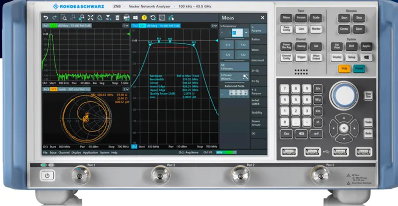
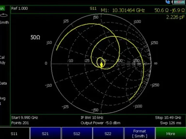
A vector network analyzer measures the reflection characteristics of an RF component or network. For a single-port antenna measurement, the analyzer typically measures S11 over a selected frequency range.
A Smith Chart display can then show the impedance associated with the measured reflection coefficient, provided the instrument uses the correct reference impedance and calibration settings.
A typical measurement procedure includes the following steps:
Step 1: Configure the frequency range. Select a sweep that covers the antenna’s intended operating band. For example, a 2.4–2.5 GHz Wi-Fi antenna can be measured over a somewhat wider range to examine its behavior around the target band.
Step 2: Calibrate the measurement system. Perform an appropriate calibration at the intended reference plane. A common single-port method uses open, short, and load standards. The standards and calibration procedure must suit the connectors, cables, and measurement setup.
Step 3: Connect the antenna. Attach the antenna to the calibrated test system, maintaining a consistent setup and avoiding unnecessary cable movement.
Step 4: Select the measurement display. Configure the analyzer to measure S11 and display the result on a Smith Chart. Set markers at important frequencies to read impedance and reflection characteristics.
Step 5: Evaluate the results. Examine the impedance trajectory across the frequency range rather than judging the antenna from a single frequency point.
The exact menu names vary between VNA models, so the procedure should be adapted to the instrument’s documentation.
6.2 How to Interpret Antenna Measurement Results
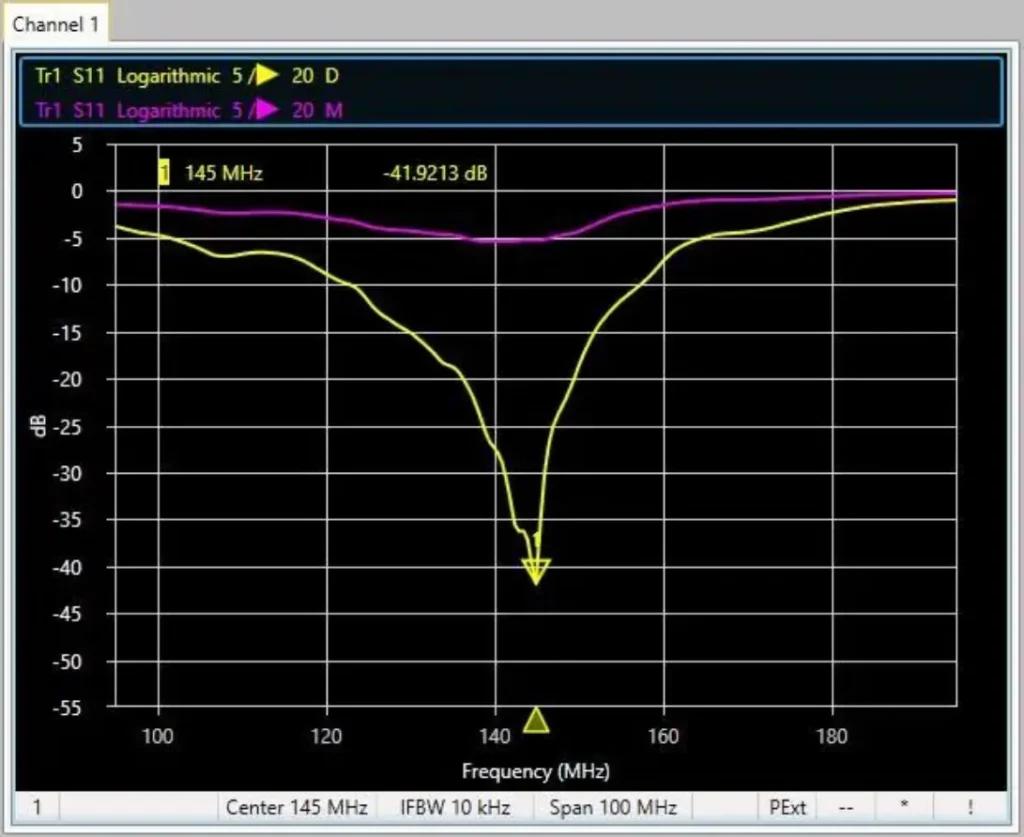
The Smith Chart shows how the antenna’s input impedance changes with frequency. A point closer to the chart center generally indicates a closer match to the reference impedance at that frequency.
Engineers commonly use the chart alongside S11, return loss, and VSWR to evaluate matching performance.
For a conventional real reference impedance, the relationship between S11 magnitude and return loss is:
RL = −20 log₁₀|S₁₁| dB
A more negative S11 value in dB generally indicates less reflected power, while a larger positive return loss indicates a better match.
However, impedance matching is only one aspect of antenna performance. A low VSWR does not, by itself, prove that an antenna has high radiation efficiency, high gain, or a desirable radiation pattern. Those characteristics require additional measurements or simulations.
For this reason, engineers should combine Smith Chart analysis with other RF performance data when evaluating an antenna design.
7. Applications of the Smith Chart in Modern RF Engineering
The Smith Chart remains relevant across several areas of RF and microwave engineering.
7.1 Antenna Design and Tuning
Antenna designers use Smith Charts to inspect feed-point impedance, evaluate matching networks, and identify how impedance changes across an operating band. These insights can guide adjustments to feed structures, matching components, and antenna geometry.
7.2 RF Amplifiers and Microwave Circuits
In amplifier design, the Smith Chart helps engineers analyze input and output impedances and work with matching networks. Depending on the available device data, it can also display gain, noise, or stability contours.
These contours come from circuit measurements or models; the Smith Chart itself does not directly determine amplifier efficiency or output power.
7.3 Transmission Lines and RF Networks
The chart helps engineers calculate input impedance at different points along a transmission line and analyze impedance transformations. It is particularly useful for understanding stub matching and the relationship between electrical length and impedance.
7.4 Simulation and Automated Design
Modern RF design tools can plot impedance trajectories, calculate S-parameters, and optimize matching networks automatically. Nevertheless, understanding the Smith Chart helps engineers interpret those results, recognize unexpected impedance behavior, and make better design decisions.
Simulation and graphical analysis are complementary methods rather than competing approaches.
8. Common Smith Chart Mistakes to Avoid
Even experienced engineers need to pay attention to the reference conditions and assumptions behind a Smith Chart.
Confusing Actual and Normalized Impedance
A Smith Chart’s impedance grid normally displays normalized values. Engineers must divide the actual impedance by the reference impedance before plotting it, then multiply by the reference impedance to recover the actual value.
Mixing Up Open, Short, and Matched Points
The center represents a match, the rightmost point represents an open circuit, and the leftmost point represents a short circuit. All three conditions have distinct impedance and reflection coefficient values.
Assuming Low VSWR Guarantees Good Antenna Performance
VSWR describes the degree of impedance matching at the measurement reference plane. It does not independently measure radiation efficiency, gain, polarization, or coverage.
Ignoring Frequency and Measurement Conditions
Impedance can change significantly with frequency. Cable losses, connector quality, calibration errors, and the chosen reference plane can also affect measurements. Engineers should therefore verify performance under the intended operating conditions.
Applying Series and Shunt Rules to the Wrong Representation
Series reactances are straightforward to analyze on an impedance Smith Chart. Parallel reactive components are often easier to analyze on an admittance chart. Mixing the two representations can lead to incorrect component values or movement directions.
Conclusion
The Smith Chart remains one of the most useful graphical tools in RF engineering because it connects complex impedance, reflection coefficient, and transmission line behavior in a single representation.
By understanding normalized impedance, constant resistance circles, constant reactance arcs, and VSWR circles, engineers can interpret impedance measurements and develop effective matching networks. The same principles apply to antenna tuning, amplifier design, and transmission line analysis.
Modern simulation software and VNAs make calculations faster, but a sound understanding of the Smith Chart helps engineers interpret results and make more informed design decisions. Combining graphical analysis with accurate measurements and simulation provides a practical foundation for developing reliable RF systems.
At Airplux Technologies, antenna performance and impedance matching are important considerations in developing customized antenna solutions for different RF applications. Understanding these fundamentals helps engineers evaluate antenna interfaces, identify matching requirements, and work toward reliable performance across the intended operating band.
You may also like
Master VSWR vs Return Loss — how they indicate mismatch, reflected power, and why both matter in RF antenna systems.

Learn what antenna efficiency means, how radiation and total efficiency differ, and how VSWR and gain affect antenna performance.

Learn what is antenna polarization, its types, importance, and applications in modern wireless communication systems.

Learn what antenna gain means, how gain relates to directivity and efficiency, how dBi and dBd differ, and how to Choose the Right Gain.
Contact
We are always ready to serve you.
Please feel free to contact us
for any antenna inquiry or requirement.
Leave us a message in the form below and
we will get back to you within 24 hours.